Tank Gauge Accuracy:¶

1. what is the accuracy of these sensors?¶

MTS LT420 analog level transmitter¶

Each benchmark station (excluding Primet) has a “Stand Alone” raing gauge, consisting of a collection tank with a stand pipe in parallel, where tank level is measured. Additionally, 2 stations have a shelter top rain gauge that funnels water to a measurement/storage tank. In both designs, the tank/stand-pipe depth is measured using an analog level transmitter (magnetorestrictive), and the storage tank has a smaller area than the orifice, increasing sensitivity to small rainfall events.

2 of these appear to be malfunctioning, intermitently. A replacement must be found that has comparable accuracy, precision, and dependability. So, the first question is:

What is the accuracy of this sensor?

Must account for ratio of orifice to tank.

Sensor	% Repeatable	Range	Measurement Precision	Precip Precision	Accuracy	Precip Accuracy
MTS LT420 (SA)	0.01%	113”	0.0113” (0.287 mm)	0.00316” (0.080mm)	0.035%	0.011” (0.28 mm)
MTS LT420 (SH)	0.01%	54”	0.0053” (0.135 mm)	0.00441” (0.112mm)	0.035%	0.015” (0.3810 mm)
MTS LPR (new)	0.001%	113”	0.00113” (0.0287 mm)	0.000316” (0.0080mm)	0.039” (1 mm)	0.0109”(0.277 mm)

Based on this, we should only report to 0.1 mm. We report one additional decimal place, which seems standard.

2. What accuracy do we claim in metadata?¶

I can’t find this reported anywhere.

3. Have we been observing that accuracy?¶

First we’ll have to load a lot of instantaneous tank measurements.

[3]:

# import analysis packages
import pandas as pd
import matplotlib.pyplot as plt
import os
from glob import glob
from numpy import random

# Jupyter magic to display plots inline
%matplotlib inline
# expand all plots to comfortable viewing size
plt.rcParams['figure.figsize'] = [15, 10]

# custom MET functions
import sys
sys.path.append("../verify/")
from verify import *

[16]:

ppt_merge = met_func.CompareData('PPT')
ppt_merge.add_provisional_data('c:/workspace/LevelRainGauge\\and_precipcomps_15min.csv')
print 'Warning from QA to catch long strings in rows (in this case, DataSetName)'

ppt_merge.df.columns

Warning: File is not CSV delimited
No delimeter found

Warning from QA to catch long strings in rows (in this case, DataSetName)

[16]:

Index([u'DataSetName', u'Site', u'PRIMET_PRECIP_TOT_100_0_01',
       u'CENMET_PRECIP_INST_455_0_01', u'CENMET_PRECIP_TOT_455_0_01',
       u'CENMET_PRECIP_INST_625_0_02', u'CENMET_PRECIP_TOT_625_0_02',
       u'UPLMET_PRECIP_INST_625_0_02', u'UPLMET_PRECIP_TOT_625_0_02',
       u'UPLMET_PRECIP_INST_455_0_01', u'UPLMET_PRECIP_TOT_455_0_01',
       u'VARMET_PRECIP_INST_455_0_02', u'VARMET_PRECIP_TOT_455_0_02',
       u'CS2MET_PRECIP_INST_250_0_02', u'CS2MET_PRECIP_TOT_250_0_02'],
      dtype='object')

Yay Adam! Merged file is great!

Behavior when QC thinks it’s raining¶

So, now let’s select all the times where it wasn’t raining

Known functioning case: CENT¶

We’ll start with CENT because we don’t think either of the tank gauges have malfunctioned. This will be our baseline precision. However, winter of 2015-2016 and fall of 2017 the SA froze, plus there are some kown clogs from spring of 2019. For this reason the analysis will start with the shelter for now.

[18]:

cent_sh = met_func.CompareData('CENT SH')
cent_sh.df = ppt_merge.df[['CENMET_PRECIP_INST_625_0_02',
                       u'CENMET_PRECIP_TOT_625_0_02']]

delta_tank = cent_sh.df.CENMET_PRECIP_INST_625_0_02.diff()
not_raining = cent_sh.df.CENMET_PRECIP_TOT_625_0_02 == 0
tank_no_rain = delta_tank[not_raining]

# I couldn't stand to copy and paste this anymore
def ppt_assess(ppt, tank, date, drain_size=-2.75):
    '''
    Assess variation in sensor readings during "no rain" conditions

    :param ppt: precipitation data series
    :param tank: instantaneous tank measurement data series
    :param drain_size: keyword argument. Depth used to filter out tank
                       drains
    :param date: list containing 2 strings, a start and finish date
    :return: data series of tank measurements with tank drains and precip
             amount masked.
    '''
    not_raining = ppt == 0
    delta_tank = tank.diff()

    tank_no_rain = delta_tank[not_raining]
    tank_no_rain_no_drain =  tank_no_rain[tank_no_rain > drain_size]

    start = date[0]
    finish = date[1]
    # plot
    #plt.hold('on')
    plt.subplot(3,1,1)
    tank.loc[start:finish].plot()
    plt.grid('on')
    #plt.hold('on')
    plt.subplot(3,1,2)
    ppt.loc[start:finish].plot()
    plt.grid('on')
    #plt.hold('on')
    plt.subplot(3,1,3)
    tank_no_rain_no_drain.loc[start:finish].plot(linestyle='', marker='.')
    plt.grid('on')
    #plt.hold('on')

    return tank_no_rain_no_drain

# print tank_no_rain.loc['12/30/17']
# print cent_sh.df.loc['12/30/17']

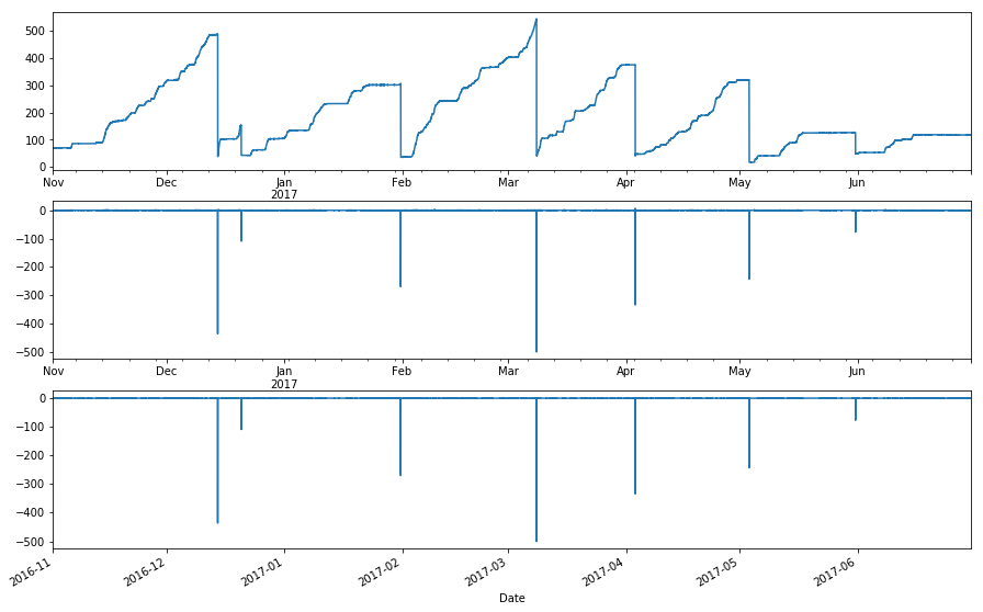
# SPOT check
plt.subplot(3,1,1)
cent_sh.df.CENMET_PRECIP_INST_625_0_02.loc['Nov 2016':'Jun 2017'].plot()
plt.subplot(3,1,2)
delta_tank.loc['Nov 2016':'Jun 2017'].plot()
plt.subplot(3,1,3)
tank_no_rain.loc['Nov 2016':'Jun 2017'].plot()

[18]:

<matplotlib.axes._subplots.AxesSubplot at 0x1fcd9898>

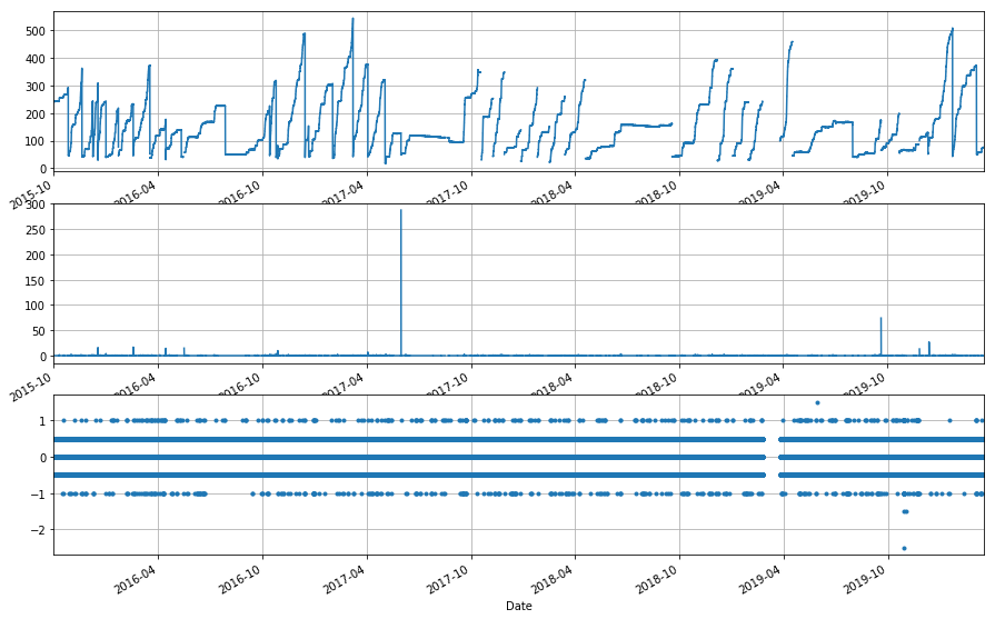
Filter out drains¶

So obviously it’s working, but we need a threshold for filtering drains out of the dataset. The merged datasets don’t have any flags. Maybe if we accessed this a different way we could just grab flags.

Lets start with 100, and see if that works for out dataset.

[5]:

tank_no_rain = delta_tank[not_raining]
tank_no_rain_no_drain = tank_no_rain[tank_no_rain>-10]

# SPOT check
plt.subplot(3,1,1)
cent_sh.df.CENMET_PRECIP_INST_625_0_02.loc['Nov 2016':'Jun 2017'].plot()
plt.subplot(3,1,2)
delta_tank.loc['Nov 2016':'Jun 2017'].plot()
plt.subplot(3,1,3)
tank_no_rain_no_drain.loc['Nov 2016':'Jun 2017'].plot()

[5]:

<matplotlib.axes._subplots.AxesSubplot at 0x22ef5898>

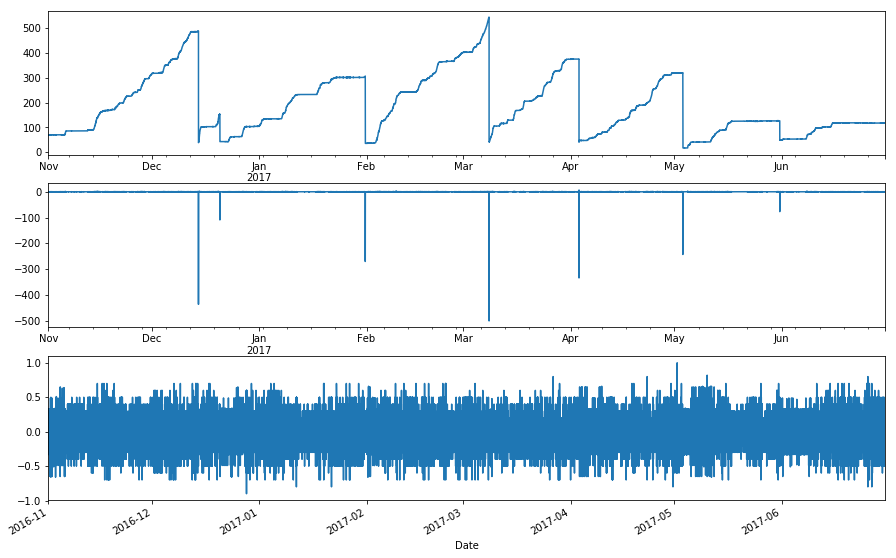
With a little iteration, -10 filters out all of the drains. For the first test period, it doesn’t seem to exclude any other data points. The next step is to test over the whole data period and see if this accidentally filters data we don’t want it to.

[19]:

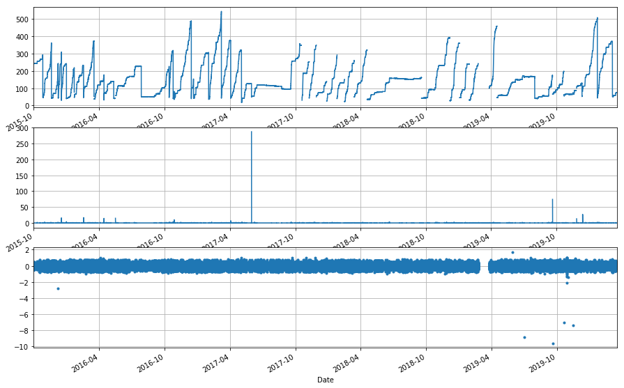
# SPOT check
_ = ppt_assess(cent_sh.df.CENMET_PRECIP_TOT_625_0_02, cent_sh.df.CENMET_PRECIP_INST_625_0_02, ['2014','2020'], drain_size=-10)

[41]:

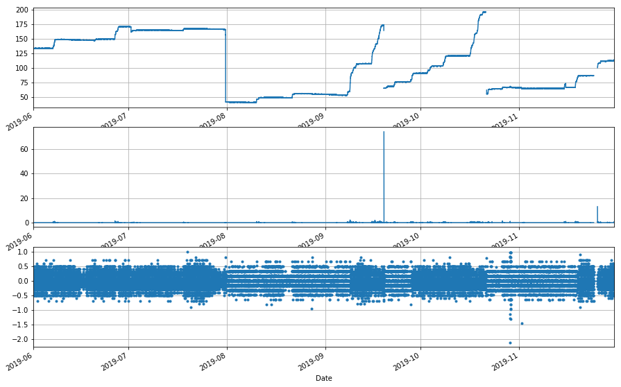
_ = ppt_assess(cent_sh.df.CENMET_PRECIP_TOT_625_0_02, cent_sh.df.CENMET_PRECIP_INST_625_0_02, ['Jun 2019','Nov 2019'], drain_size=-6)

O.K., so we’re not excluding any pertinent data, but we are still including a few drains, which look like they’re probably an order of magnitude bigger than the standard bounce, so let’s cut those out so that we don’t skew our analysis.

Note

For some reason, most of the data from WY2018 on has NAN values during drains. Not sure what QA process is doing this, or why 8 or so are missed. Maybe it’s a part of the merge

[42]:

tank_no_rain_no_drain = tank_no_rain[tank_no_rain>-2.75]

# SPOT check
plt.subplot(3,1,1)
cent_sh.df.CENMET_PRECIP_INST_625_0_02.plot()
plt.subplot(3,1,2)
delta_tank.plot()
plt.subplot(3,1,3)
tank_no_rain_no_drain.plot(linestyle='', marker='.')

[42]:

<matplotlib.axes._subplots.AxesSubplot at 0x7b247b38>

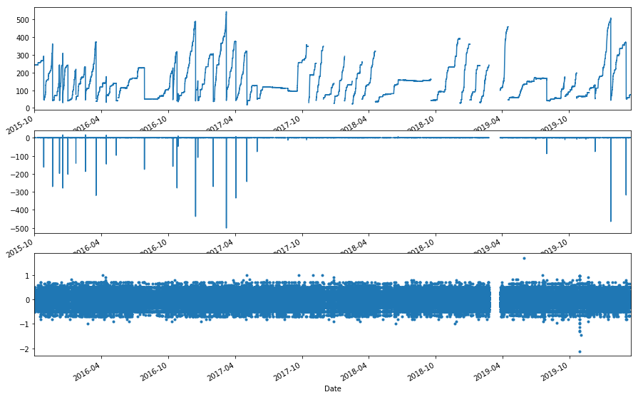
Variation in measurements¶

[44]:

print tank_no_rain_no_drain.describe()
tank_no_rain_no_drain.hist(bins=30)
plt.figure()
plt.boxplot(tank_no_rain_no_drain)
plt.grid('on')

count    424377.000000
mean         -0.002935
std           0.192207
min          -2.120000
25%          -0.100000
50%           0.000000
75%           0.100000
max           1.700000
Name: CENMET_PRECIP_INST_625_0_02, dtype: float64

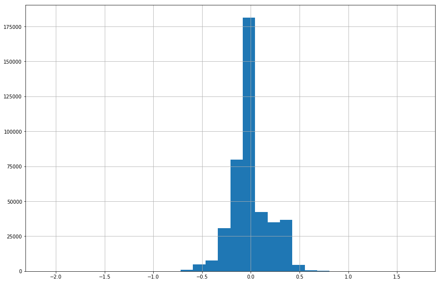
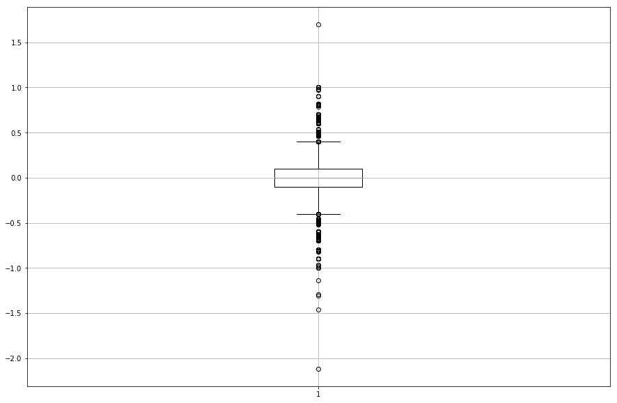
That’s great! We expect the true difference between all measurements during rain free periods to be 0, and our mean difference was very close (-0.0029 mm), which is 3 orders of magnitude below the sensors stated accuracy. The precision we have observed, however, +-0.2mm, is double expected precision. All together, error is about half of the expexted combined error.

I think this means that, yes, we have seen this level of precision in our measurements and need to find a replacement that will maintain this precision.

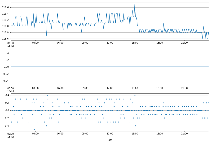
Let’s check a single day to make sure this makes sense.

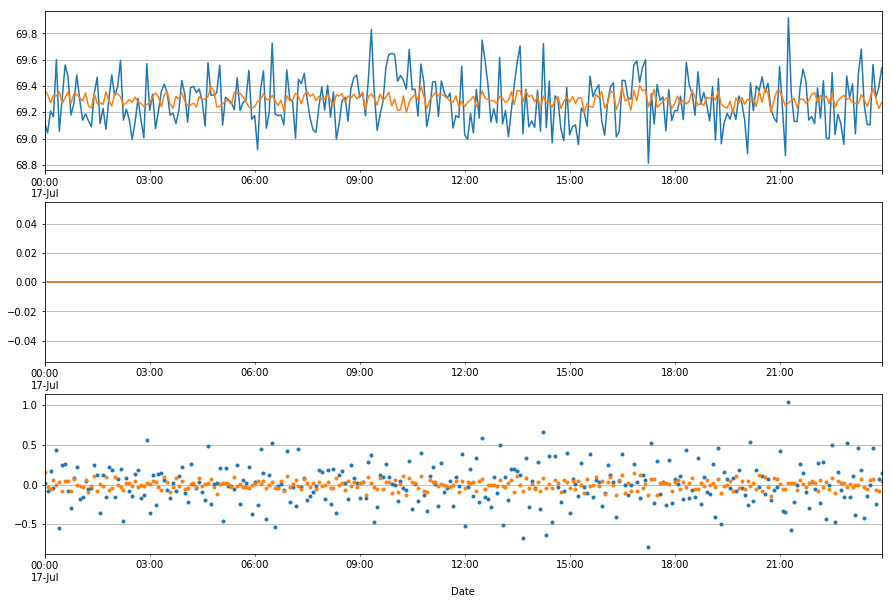
Dry Day¶

[8]:

plt.subplot(3,1,1)
cent_sh.df.CENMET_PRECIP_INST_625_0_02.loc['7/13/17'].plot()
plt.grid('on')
plt.subplot(3,1,2)
cent_sh.df.CENMET_PRECIP_TOT_625_0_02.loc['7/13/17'].plot()
plt.grid('on')
plt.subplot(3,1,3)
tank_no_rain_no_drain.loc['7/13/17'].plot(linestyle='', marker='.')
plt.grid('on')

Wet Day¶

[9]:

plt.subplot(3,1,1)
cent_sh.df.CENMET_PRECIP_INST_625_0_02.loc['11/13/17'].plot()
plt.grid('on')
plt.subplot(3,1,2)
cent_sh.df.CENMET_PRECIP_TOT_625_0_02.loc['11/13/17'].plot()
plt.grid('on')
plt.subplot(3,1,3)
tank_no_rain_no_drain.loc['11/13/17'].plot(linestyle='-', marker='.')
plt.grid('on')

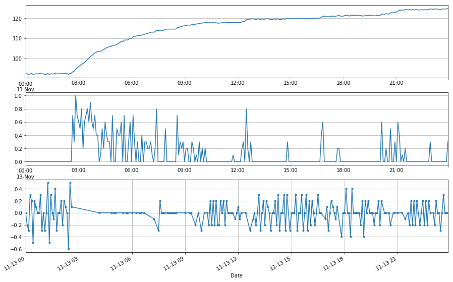
This seems to highlight a different problem. While the average variation, or repeatablitiy, between 2 measurments, taken 5 minutes apart, is around 0.2 mm (just under 0.01”), the trend is often cumulative in one direction and then another over 15-30 minutes.

Precision across sites¶

We go through them individually below, but SA seems about twice as precise as shelter rain gauges. Happily, all of the sites we think are working right all turn out to have about the same precision, accuracy, and total error.

CENT SA¶

[75]:

cent_sa = met_func.CompareData('CENT SA')
cent_sa.df = ppt_merge.df[['CENMET_PRECIP_INST_455_0_01',
                           u'CENMET_PRECIP_TOT_455_0_01']]

sa_diff = ppt_assess(cent_sa.df.CENMET_PRECIP_TOT_455_0_01,
                     cent_sa.df.CENMET_PRECIP_INST_455_0_01, ['2014', '2020'], -2.75)
sa_diff.describe()

[75]:

count    406741.000000
mean         -0.001079
std           0.086075
min          -2.500000
25%           0.000000
50%           0.000000
75%           0.000000
max           2.010000
Name: CENMET_PRECIP_INST_455_0_01, dtype: float64

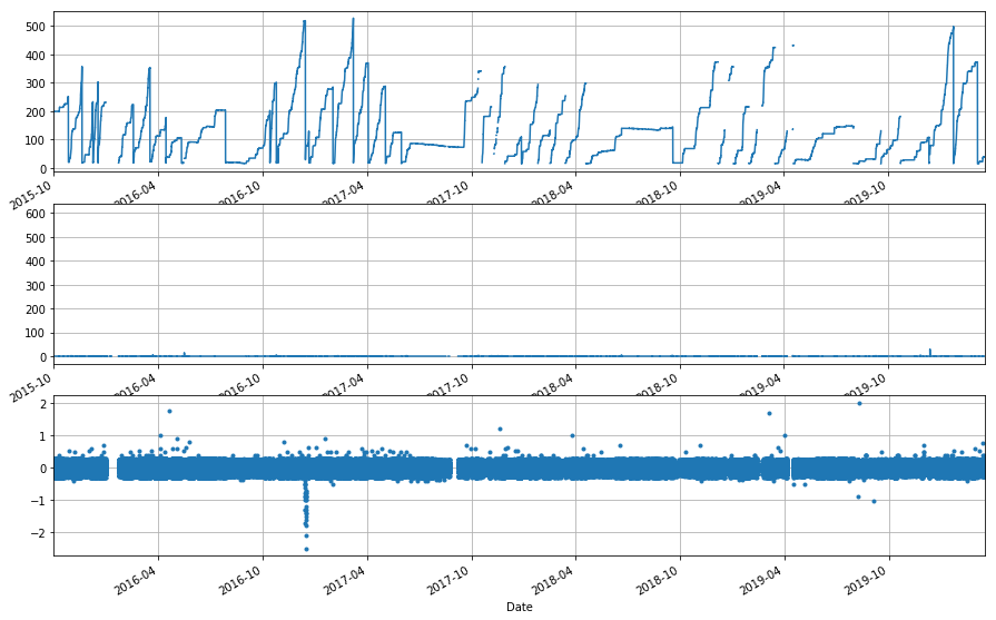
The stand alone is about twice as precise and twice as accurate. That’s great.

UPLO SA¶

This is the last sensor we know for sure to work.

[76]:

tank = ppt_merge.df['UPLMET_PRECIP_INST_455_0_01']
ppt =  ppt_merge.df['UPLMET_PRECIP_TOT_455_0_01']

sa_diff = ppt_assess(ppt, tank, ['2014', '2020'], -2.75)
sa_diff.describe()

[76]:

count    393470.000000
mean         -0.001509
std           0.083516
min          -2.000000
25%          -0.060000
50%           0.000000
75%           0.040000
max           2.300000
Name: UPLMET_PRECIP_INST_455_0_01, dtype: float64

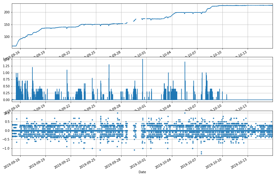
UPLO SH¶

We know there were some problems here. I guess they aught to show up if we’re doing this right.

This is pretty underwhelming. We mostly seem to be unable to capture the problem. I iterated over multiple time scales, with multiple drain thresholds. Only thing I can really say is that UPLO has a slightly increased SD and mean diff.

2014-2020; drain threshold of -100

mean -0.005980

std 0.452126

VARA is even worse, though I think this is mostly because of data that just had nan’s applied.

[19]:

tank = ppt_merge.df['UPLMET_PRECIP_INST_625_0_02']
ppt =  ppt_merge.df['UPLMET_PRECIP_TOT_625_0_02']

sa_diff = ppt_assess(ppt, tank, ['Sept 15, 2019', 'Oct 15, 2019'], -100)
sa_diff.describe()

C:\WinPython-64bit-2.7.10.3\python-2.7.10.amd64\lib\site-packages\matplotlib\cbook\deprecation.py:107: MatplotlibDeprecationWarning: Passing one of 'on', 'true', 'off', 'false' as a boolean is deprecated; use an actual boolean (True/False) instead.
  warnings.warn(message, mplDeprecation, stacklevel=1)

[19]:

count    327765.000000
mean         -0.005980
std           0.452126
min         -94.400000
25%          -0.100000
50%           0.000000
75%           0.010000
max           2.000000
Name: UPLMET_PRECIP_INST_625_0_02, dtype: float64

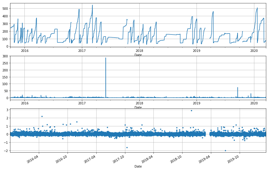
4. How much of our record has been this precise?¶

Accessing GCE files, we have a total measurement error that meets or beats the MTS made LT420 tank gauge precision of 0.27 mm. This would indicate that any replacement instrument needs to be this precise. However, that only demonstrates that we have that level of precision in the dataset for the last 5 years.

Access to raw tank measurements from earlier periods is tricky; we don’t provide raw mesurements in our datasets, formatting is inconsistent, and a lot of manual manipulation is required. Below, I try to get a glimpse into earlier periods without too much manual labor. At the very least, we know that earlier periods used a different resistor as a shunt, which would impact measurements.

[171]:

# # get a list of file paths that have 5 min instantaneous data
# start analysis on CENT since it has the both instruments on the same logger

def scour_4_edlog_data(folder, name):
    # WARNING!!!! This is super inefficient, BAD coding.
    # Yuck, super embarassing. Just busting through this thing
    subdir = os.listdir(folder)
    in_dir = []
    for f in subdir:
        if f.isdigit():
            subsubdir = folder + '/' + f
            for name in os.listdir(subsubdir):
                name_low = name.lower()
                abspath = subsubdir + '/' + name
                if name_low.endswith('5min.csv') and not '1' in name_low:
                    in_dir.append(abspath)
                    break
                # elif name.endswith('.dat') and not any(n in name for n in ['233','SYS','PWR', 'CONT']) and 'Table105' in name:
                #     in_dir.append(abspath)
                #     break

    # load all .csv files and modern .dat files (toa5)
    site = met_func.CompareData(name)
    for n in in_dir:
        if n.endswith('.dat'):
            site.add_toa5_data(n)
        else:
            csv = pd.read_csv(n, parse_dates=['date'])

            time_fn = csi.CampbellData().get_cr10_to_HHMM
            csv['J'] = csv.date.dt.strftime('%j')
            csv['Y'] = csv.date.dt.strftime('%Y')
            date_formatted = time_fn(csv[['J', 'time', 'Y']])
            ts = pd.to_datetime(date_formatted, format='%Y %j %H%M')
            csv= csv.set_index(ts)

            df = site.merge_data(site.df, csv)
            site.df = df

    return site, in_dir

folder = '\server\UPLO'
name = 'UPLO_Precip'

uplo, indir = scour_4_edlog_data(folder, name)

[206]:

uplo.df.tail()

[206]:

	J	Y	date	orificesa	orificesh	precipsa	precipsh	quality	snowdep	snowmois	time
2004-12-31 23:40:00	366	2004	2004-12-31	4.61	20.74	156.9	122.3	-280.0	285.0	85.2	2340
2004-12-31 23:45:00	366	2004	2004-12-31	4.40	21.31	156.9	122.1	-290.0	293.0	85.5	2345
2004-12-31 23:50:00	366	2004	2004-12-31	4.05	22.09	156.9	122.3	0.0	5600.0	85.5	2350
2004-12-31 23:55:00	366	2004	2004-12-31	4.58	22.49	156.9	122.3	-281.0	287.0	85.5	2355
2005-01-01 00:00:00	366	2004	2004-12-31	4.19	21.76	156.9	122.2	-286.0	287.0	85.5	2400

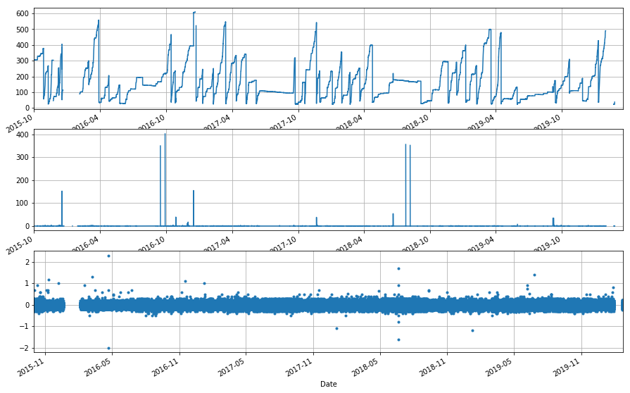
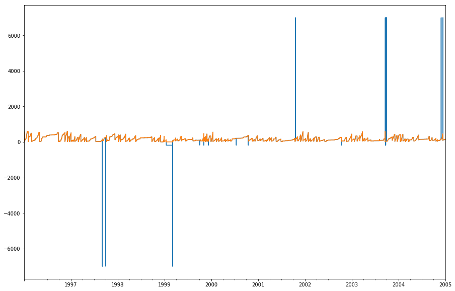
[207]:

uplo.df.head()
del sa
sa = uplo.df.precipsa
sa.plot()

tank_spike_filter = sa[(sa>0)&(sa<600)]
tank_spike_filter.plot()

delta_tank = tank_spike_filter.diff()
plt.figure()
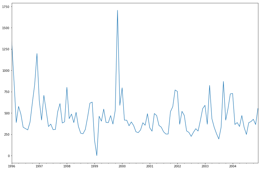
delta_tank[delta_tank>0].plot()

mly = delta_tank[delta_tank>0].resample('1M').sum()
plt.figure()
mly.plot()

[207]:

<matplotlib.axes._subplots.AxesSubplot at 0x10ad171d0>

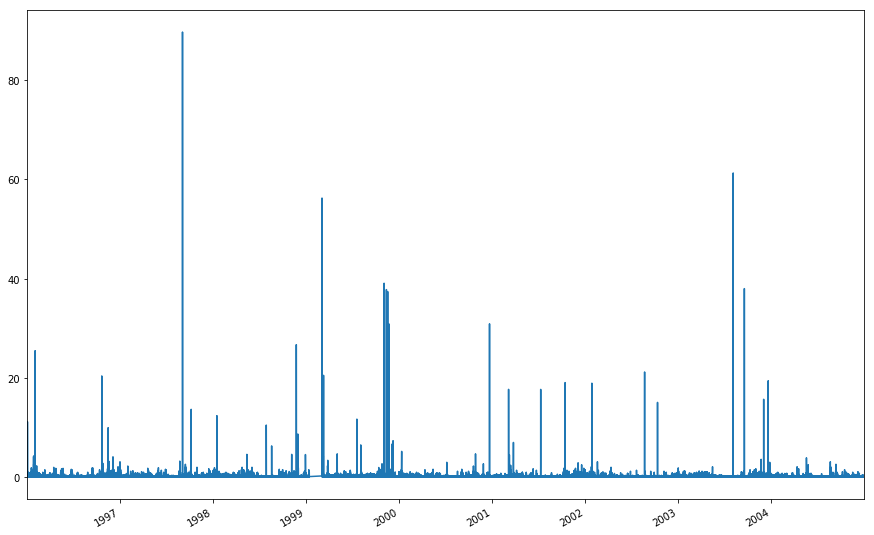
[250]:

ms01 = load_data.MergeData()
ms01.add_ms001_data('c:/DATA\MS001_dwnld\UPLO_SA_1994-2004_5min.csv')
uplo_ppt = pd.to_numeric(ms01.df.PRECIP_TOT, errors='coerce')

tank_spike_filter = tank_spike_filter.loc[uplo_ppt.index]
sa_diff = ppt_assess(uplo_ppt, tank_spike_filter, ['1995', '2004'], -10)

sa_diff.describe()

C:\WinPython-64bit-2.7.10.3\python-2.7.10.amd64\lib\site-packages\ipykernel\__main__.py:2: DtypeWarning: Columns (4) have mixed types. Specify dtype option on import or set low_memory=False.
  from ipykernel import kernelapp as app

[250]:

count    777588.000000
mean          0.005089
std           0.295359
min          -9.750000
25%           0.000000
50%           0.000000
75%           0.000000
max          89.700000
Name: precipsa, dtype: float64

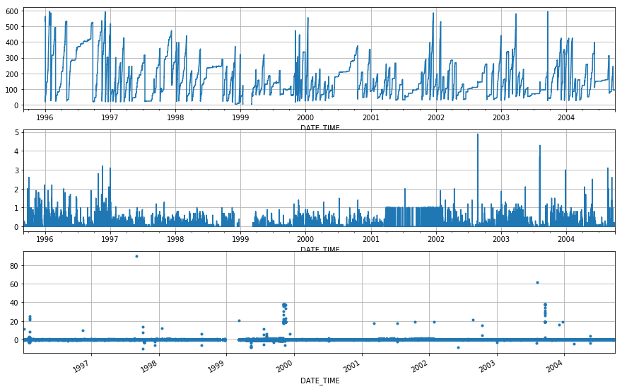
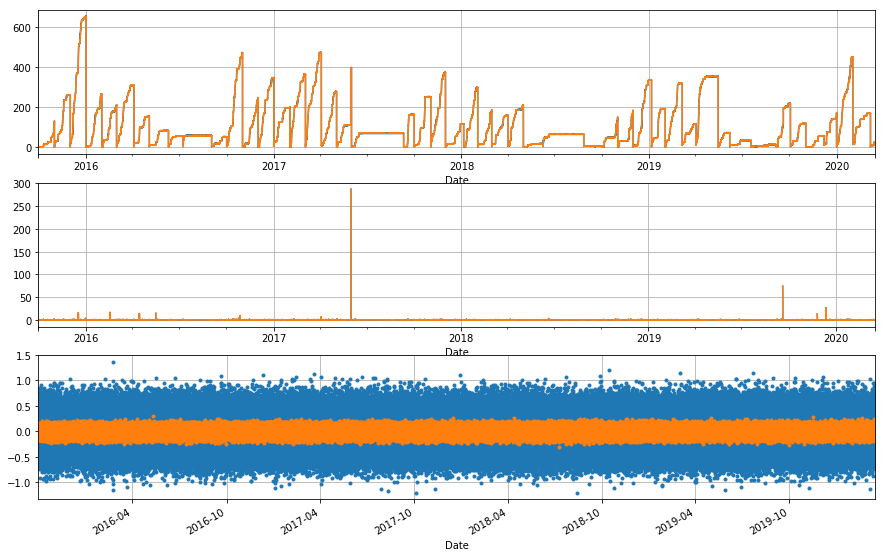
Ok, so the formatting’s a nightmare, but the precision is surprisingly good. The mean accuracy is 5x worse, but is still < 0.01 mm. And the SD (precision) is about 3x worse. A quick visual scan suggests this may be driven by some outliers that may have had manual QC at some stage. However, this is still nearly, or below, 0.01” total measurment error. So even on older model loggers and their associated limitations in data formatting, the accuracy was on average +- < 0.01 mm and the precision in our measurments was generally 0.3 mm. This confirms that data at the HJ has been at least within sensor specified instrument error for almost all of our record, so any repairs or replacements need to be 0.01” or better.

The data takes a lot of manipulation, and individual MS0X downloads, so I’m not going to test any other sites here. The method above can be reapplied if someone else wants to do some testing.

Possible improvements to measurement¶

Possible ways to improve this include:

Taking median float position instead of instantaneous
Rounding everything to 0.5 mm
Smoothing the float to a larger time step

Average- down sample from 5min¶

[10]:

tank_15min_mean = cent_sh.df.CENMET_PRECIP_INST_625_0_02.resample('15min').mean()
delta_tank15 = tank_15min_mean.diff()

ppt_15min = cent_sh.df.CENMET_PRECIP_TOT_625_0_02.resample('15min').sum()
not_raining = ppt_15min == 0
tank_no_rain15 = delta_tank15[not_raining]

tank_no_rain_no_drain15 = tank_no_rain15[tank_no_rain15>-2]


plt.subplot(3,1,1)
tank_15min_mean.loc['7/13/17'].plot()
plt.grid('on')
plt.subplot(3,1,2)
ppt_15min.loc['7/13/17'].plot()
plt.grid('on')
plt.subplot(3,1,3)
tank_no_rain_no_drain15.loc['7/13/17'].plot(linestyle='-', marker='.')
plt.grid('on')
plt.suptitle('Averaged Tank Level (3 samples/15min)')

[10]:

Text(0.5,0.98,'Averaged Tank Level (3 samples/15min)')

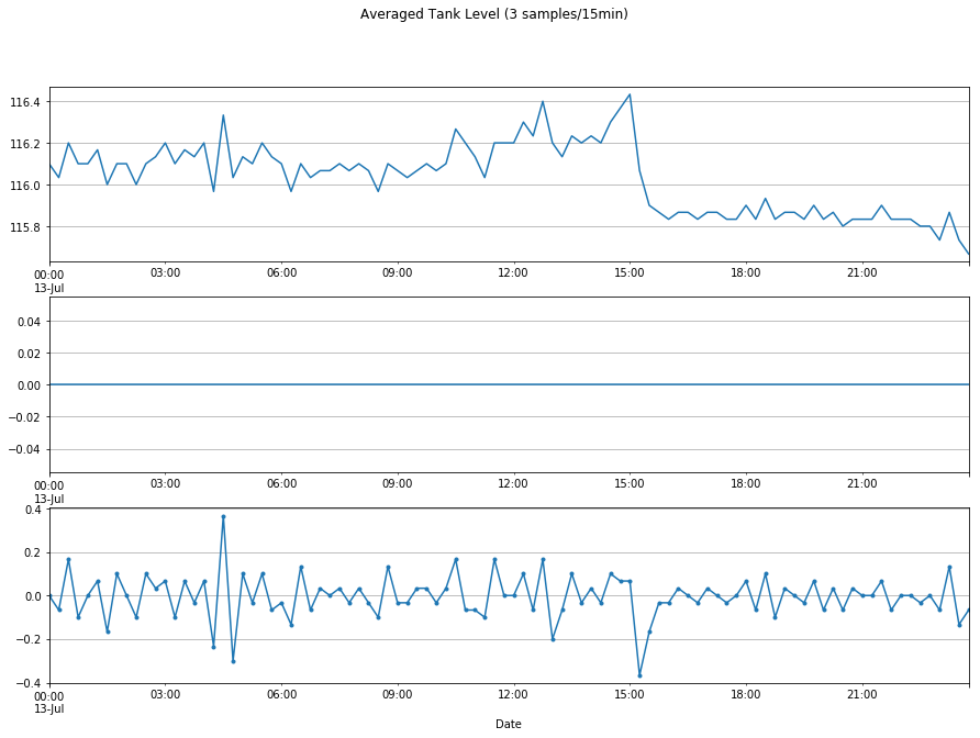
So that didn’t do a lot…So, if we implemented at the logger, instead of just averaging 3 points, we could average 20 points every 5 minutes. Let’s see what that would look like. 20 points, would be a 90 min average on the data downstream from the logger.

Let’s stick to an hour, or 20 measurements.

[45]:

tank_4hr = cent_sh.df.CENMET_PRECIP_INST_625_0_02.resample('1H').mean()
ppt4hr = cent_sh.df.CENMET_PRECIP_TOT_625_0_02.resample('1H').sum()

filtered4hr_tank = ppt_assess(ppt4hr, tank_4hr, ['7/13/17','7/13/17'],-2)
plt.figure()
ppt_assess(ppt4hr, tank_4hr, ['2013','2020'],-2)

filtered4hr_tank.describe()

[45]:

count    29290.000000
mean         0.007430
std          0.091348
min         -1.979167
25%         -0.041667
50%          0.000000
75%          0.050000
max          2.883333
Name: CENMET_PRECIP_INST_625_0_02, dtype: float64

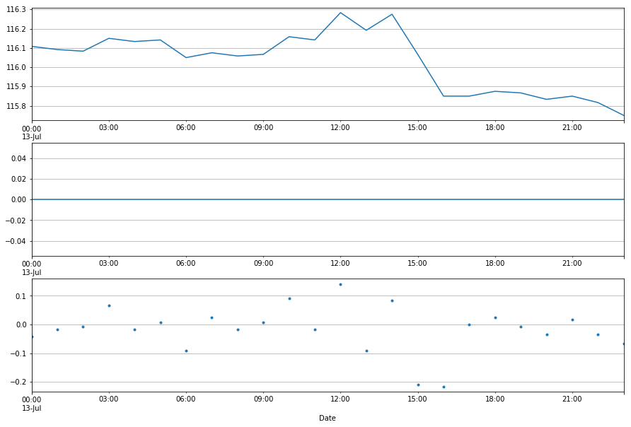
At an hour bassis that’s a pretty notable improvement. The mean doubled from 0.003 mm to 0.007 mm, however the interquartile range and standard deviation were cut in half. I think that in this application, the increase in precision (reduced SD) makes up for the decrease in accuracy (increased mean) because the combined instrument error is reduced. I’m going to take one last crack at simulating what this shift would be like at the sensor level.

Average- upsample to synthetic 15 sec data¶

I’ll use the precip to create a smoothed, synthetic tank level. I’ll then fuzzy this synthetic tank with a random number generator proportional to the mean and standard deviation. Unfortunately I can’t up sample the tank level, because I don’t have a way to rerun the QA process and recalculate precip…

mean -0.00293

std 0.19218

[55]:

avg = -0.00293
std = 0.19218

def apply_cumsum(df):
    return df.cumsum()

# take the cum sum of the monthly groups
mthly = cent_sh.df.CENMET_PRECIP_TOT_625_0_02.resample('1m')
cum_ppt_mthly = mthly.agg(apply_cumsum)

# upsample to 15 sec with a forward fill
syn_tank_scan_smooth = cum_ppt_mthly.drop_duplicates().resample('15S').ffill()
print 'upsample 5 min to 15 sec\n'
print syn_tank_scan_smooth.tail()

# add a random number where the average randome number is the average variance and the distribution is spread by 1SD
# use of apply is slower than generating a second array and adding the 2
# syn_tank_meas_var = syn_tank_meas_smooth.apply(lambda x: x + random.normal(loc=avg, scale=std))
syn_tank_scan_var = syn_tank_scan_smooth + random.normal(loc=avg, scale=std, size= len(syn_tank_scan_smooth))
print '\nAdd sensor bounce from radom num w/ 0.19mm stdev'
print syn_tank_scan_var.tail()

syn_tank_5min_grp = syn_tank_scan_var.resample('5min')

syn_tank_5min_mean = syn_tank_5min_grp.mean()
print '\nReseample to 5min mean of 15 sec scan'
print syn_tank_5min_mean.tail()

syn_tank_5min_smpl = syn_tank_5min_grp.last()
print '\nResample to 5min by sampling last value'
print syn_tank_5min_smpl.tail()

# So this was more than an hour of complicated trouble shooting, but
# 10/1/XXXX 00:00 is repeated multiple times in the merge file
# this was allowing slicing, until I resampled and the duplicates only
# existed on one side of the slice (i.e. tank[no_rain] had different
# lengths and indexes). Also, if you drop duplicates on a cumsum, it
# drops every 5 min period where it wasn't raininng and cumsum was stable
ppt = cent_sh.df.CENMET_PRECIP_TOT_625_0_02.loc[~cent_sh.df.index.duplicated()]
plt.clf()
smpled_tank_diff = ppt_assess(ppt, syn_tank_5min_smpl, ['2013','2020'],-2.75)
plt.hold('on')
avged_tank_diff = ppt_assess(ppt, syn_tank_5min_mean, ['2013','2020'],-2.75)

print smpled_tank_diff.describe()
avged_tank_diff.describe()

upsample 5 min to 15 sec

Date
2020-03-16 16:09:00    25.62
2020-03-16 16:09:15    25.62
2020-03-16 16:09:30    25.62
2020-03-16 16:09:45    25.62
2020-03-16 16:10:00    25.67
Freq: 15S, Name: CENMET_PRECIP_TOT_625_0_02, dtype: float64

Add sensor bounce from radom num w/ 0.19mm stdev
Date
2020-03-16 16:09:00    25.622975
2020-03-16 16:09:15    25.350635
2020-03-16 16:09:30    26.038003
2020-03-16 16:09:45    25.792657
2020-03-16 16:10:00    25.591394
Freq: 15S, Name: CENMET_PRECIP_TOT_625_0_02, dtype: float64

Reseample to 5min mean of 15 sec scan
Date
2020-03-16 15:50:00    25.619421
2020-03-16 15:55:00    25.578160
2020-03-16 16:00:00    25.561200
2020-03-16 16:05:00    25.540448
2020-03-16 16:10:00    25.591394
Freq: 5T, Name: CENMET_PRECIP_TOT_625_0_02, dtype: float64

Resample to 5min by sampling last value
Date
2020-03-16 15:50:00    25.834310
2020-03-16 15:55:00    25.369554
2020-03-16 16:00:00    25.586378
2020-03-16 16:05:00    25.792657
2020-03-16 16:10:00    25.591394
Freq: 5T, Name: CENMET_PRECIP_TOT_625_0_02, dtype: float64
count    433203.000000
mean          0.000073
std           0.272089
min          -1.209440
25%          -0.183282
50%          -0.000213
75%           0.183412
max           1.365707
Name: CENMET_PRECIP_TOT_625_0_02, dtype: float64

C:\WinPython-64bit-2.7.10.3\python-2.7.10.amd64\lib\site-packages\ipykernel\__main__.py:42: MatplotlibDeprecationWarning: pyplot.hold is deprecated.
    Future behavior will be consistent with the long-time default:
    plot commands add elements without first clearing the
    Axes and/or Figure.

[55]:

count    433203.000000
mean          0.000017
std           0.060824
min          -0.310104
25%          -0.041108
50%          -0.000016
75%           0.041043
max           0.292751
Name: CENMET_PRECIP_TOT_625_0_02, dtype: float64

[51]:

plt.clf()
tdiff_smpl = ppt_assess(ppt, syn_tank_5min_smpl, ['July 17, 2017','July 17, 2017'],-2.75)
tdiff_mn = ppt_assess(ppt, syn_tank_5min_mean, ['July 17, 2017','July 17, 2017'],-2.75)

I think this is a pretty compelling case for using a mean instead of a sample. We generally use samples when data has lots of outliers, spiking dramatically in one or more directions, requiring us to filter these values to avoid skewing the data. However, this is not the case with the tank gauges. Most of our error seems to come from low precision in repeated measurments that oscilate around a mean measurement that is stable and accurate. And when they go bad, they go bad much bigger.

This data sees greatly decreased total measurement error, a great increase in accuracy, and an improvement in precision that will remove a lot of noise.

In the case of the 2 graphs above, first a cumsum of the already smoothed precip totals data was preformed. then the 15 second data was synthetically generated by using random numbers [1]. That dataset was then sampled in 2 different ways every 5 minutes: isntantaneous sample, and mean. This created a large difference in measurements from the same dataset. Especially considering they were derived from a dataset that was inherently smoothed by our post processes.

Diff between 5 min sample [2]

mean 0.000028

std 0.271703

Diff between 5 min mean

mean -0.0000003311764

std 6.067227e-02

Rounding to nearest 0.5 mm¶

[1]	Random numbers were normally distributed. The distribution had a mean and standard deviation of the differences between 5 minute measurements taken during dry periods.

[2]

In reruns of this section of code, the random number generator doesn’t seem to replicate these results precisely. This seems to simply be an artifact of the random number generator. In most reruns, the mean sampling generally has a SD 1 order of magnitude smaller, sometimes has a mean 5-10 times smaller, and the 25th and 75th percentiles, as well as the min and max, are generally 5-10 times smaller.

[71]:

def round_to_frac(number,roundto):
    return (round(number / roundto) * roundto)

tank_05round = cent_sh.df.CENMET_PRECIP_INST_625_0_02.apply(lambda x: round_to_frac(x, 0.5))
print cent_sh.df.CENMET_PRECIP_INST_625_0_02.head()
print tank_05round.head()

tank_diff_05rnd = ppt_assess(cent_sh.df.CENMET_PRECIP_TOT_625_0_02, tank_05round, ['2014','2020'], -2.75)
tank_diff_05rnd.describe()

Date
2015-10-01 00:00:00    241.3
2015-10-01 00:05:00    241.2
2015-10-01 00:10:00    241.3
2015-10-01 00:15:00    241.4
2015-10-01 00:20:00    241.2
Name: CENMET_PRECIP_INST_625_0_02, dtype: float64
Date
2015-10-01 00:00:00    241.5
2015-10-01 00:05:00    241.0
2015-10-01 00:10:00    241.5
2015-10-01 00:15:00    241.5
2015-10-01 00:20:00    241.0
Name: CENMET_PRECIP_INST_625_0_02, dtype: float64

[71]:

count    424377.000000
mean         -0.002903
std           0.260501
min          -2.500000
25%           0.000000
50%           0.000000
75%           0.000000
max           1.500000
Name: CENMET_PRECIP_INST_625_0_02, dtype: float64

Yeah, that doesn’t really help at all…

Unexplored here:¶

Does it vary with season (i.e. rainy season v.s. dry season)?
VARA and CENT SA have a horizontal pipe leaving the stand pipe well below the sensor. Is there a range (e.g. 400-500mm) where this interferes with the accumulation measurements?
What about sites that don’t use a tank gauge? CS2MET, HI15, PRIMET?

Accuracy of replacement sensors¶

Many sensors were looked at that are unsuitable. For example, during heater malfunctions the tank slushes or freezes solid around the sensor, and weather exposure to the sending unit is unavoidable. Precision has historically been similar to the CS2MET and Primet gauges, ~0.01”, but few tank gauges meet this requirement.

The table includes key examples, but other sensors assessed include: Campbell Sci. pressure transducers (>0 C only), Omega engineering pressure transducers, Burkert guided radar, Drexelbrook tank levels, Morrison Bros. tank sensors, Madison tank sensors, ABB, etc.

The top 7 rows are currently in used in some form at HJA.

When both accuracy and precision are provided by the manufacturer, I combine them. The shelter and stand alone specific numbers represent the error to precip measurements, converting the error the sensor would measure in the tank into real precip.

Type	Sensor	Mfr	Accuracy sensor	Accuracy in SH	Accuracy in SA	$
X	Provisinoal Data	GCE		0.1951 mm	0.0872 mm
Magnetic level float	LTS (current)	MTS	1.292 mm	1.073 mm	0.3597 mm	X
Magnetic level float	LPR (new LTS)	MTS	1.029 mm	0.8549 mm	0.2864 mm	2,300
Cable level float	PAT	Stevens	2.896 mm	2.407 mm	0.8063 mm	1,150
Tipping bucket	TE525WS 8”	CSI/TXInst.	0.00254 mm [3]_	0.0009 mm	X	408
Tipping bucket	TE525 6”	CSI/TXInst.	0.00254 mm	0.0005 mm	X	376
Pressure transducer	Snotel [4]_	Druck	2.540 mm	2.111 mm	0.7072 mm	800
Pressure transducer	Automation direct	Prosense	8.767 mm	7.286 mm	2.441 mm	324
Magnetic level float	Cont. Level 0-5VDC	FPI Sensors	55.12 mm	45.18 mm	15.35 mm	Bid
Magnetic level float	Jupiter M4	Orion	1.300 mm	1.080 mm	0.3620 mm	3,657

_[3] The tipping bucekts are accurate within 1% as long as rainfall rate is < 2”/hr. Installed in the shelter, the effective max rainfall rate will be 1.7”/hr

_[4] This must first go through an extensive aging process at NRCS labs

[2]:

sa = 0.27844095497516425
sh = 0.8310968078869966

precision = .015*25.4 #(11.5*12*25.4)*0.000001
accuracy = 0.035 *25.4#(11.5*12*25.4)*0.0025
tot = precision + accuracy#1.3 #
# tipping bucket 4.73 ml v 8.24 ml
# 0.203516309571 * 0.01*(0.01 * 25.4) v 0.361806772571 * 0.01 * (0.01 * 25.4)

print tot
print tot*sa
print tot*sh

0.0038*2.5*12*25.4
0.0025*138*25.4

1.27
0.353620012818
1.05549294602

[2]:

8.763

Improvement from calculated thermal expansion¶

A replacement sensor has the potential to also measure liquid temperature. It is thought that thermal expansion accounts for some of the error in our measurement, but the amount has not been defined. To asses whether this feature is worth the cost, we need to establish some estimate of how much error it would remove.

How to calculate thermal expansion¶

This source gives a pretty good explanation, but skips over how to calculate the change in water’s coefficient of volume expansion ($\beta$). This source corroborates the prevous explanation, but also provides a table of $\beta$ and $^o$C that has been compared to the formulas used below.

Basically $\Delta V = \beta V \Delta T$

More specific equations for calculating $\beta$ from density and calculating water density from temperature were taken from multiple sources, but replicate the chart provided in the link above.

[4]:

def beta_water_expansion(T):
    '''
    https://physics.stackexchange.com/questions/56649/thermal-expansion-coefficient-of-water
    This only really works between 20 and 30 C
    '''
    return 1.6e-5 + 9.6e-6 * T

'''
def p_water_density(T):
    """
    Something's not working right here, and I can't find the reference again.
    """
    a1, a2, a3, a4, a5 = -3.983035, 301.797, 522528.9, 69.34881, 999.974950
    num = ((T + a1)**2) * ((T + a2)**2)
    denom = a3 * (T + a4)
    return a5 * (1 - num/denom)*0.001
'''

def p_water_density(t):
    '''
    https://www.ncbi.nlm.nih.gov/pmc/articles/PMC4909168/
    '''
    b, a1, a2, a3, a4, a5 = 999.83952, 16.945176, -7.9870401e-3, -46.170461e-6, 105.56302e-9, -280.54253e-12
    num = b + a1 * t + a2 * t**2 + a3 * t**3 + a4 * t**4 + a5 * t**5
    denom = 1 + 16.89785e-3 * t
    return num/denom*0.001


def beta_water(T1, T2):
    '''
    https://physics.stackexchange.com/questions/63047/calculating-the-coefficient-of-thermal-expansion-in-liquid?rq=1
    '''
    p1 = p_water_density(T1)
    p2 = p_water_density(T2)

    dP = 1/p2 - 1/p1

    dT = T2-T1
#    if dT == 0:
#        dT = 0.000000001

    return (dP/dT) * p2

T = 25
t2 = T+0.1

print beta_water_expansion(T)
print beta_water(T, t2)
print p_water_density(T)

0.000256
0.000266570572035
0.996729473867

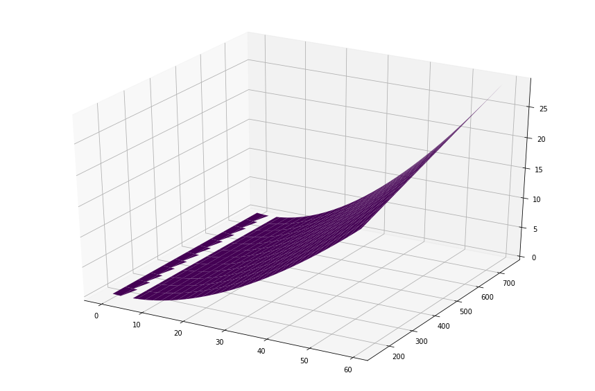
Calculating impact on measurement¶

There are 2 potential impacts of water expansion on our measurements:

Expansion is large enough to register as precip accumulation at the 5 minute record.
Over warm periods with no rain in the summer and spring, the overall tank level increases, but over a long period that is not assessed as precip by our QA processes.

I try to asses the range of possible outcomes below. The creation of false precip is the more critical concern, but the increase in tank level can be confounding as well as annoying.

A few assumptions:

The water in the tank can only expand vertically
Even though there is a volume of water below the junction between the tank and standpipe which will expand, all vertical expansion is distributed between the stand pipe and the tank
Water is always above 0 $^o$C
Comparison is always made to 4 $^o$C, which is both when water is densist, and also the temperature we heat the oriffice to, which should correlate to tank temperature because the heating pipe circulates through both areas
Assume there is always 6” of water in drain below standpipe, so stotal standpipe depth is ~700

[5]:

#%matplotlib notebook
from numpy import pi

def area_circ(d, unit='English'):
    if 'eng' in unit.lower():
        d = d * 25.4
    return pi*(d/2)**2

def delta_vol(V, t1, t2):
    beta = beta_water(t1, t2)
    dV = beta * V * (t2-t1)
    return dV

# this is the minimum head at the drain height
mindpth = 6*25.4
A = area_circ(10)+area_circ(3)

test = range(int(mindpth), 760, 50)
temp = range(0,60,1)


def gauge_response(temp, dpth):
    # this includes the tank below the stand pipe (~3.5 ft)
    V = area_circ(10)*(3.5*12*25.4 + dpth) + area_circ(3) * dpth

    A = area_circ(10)+area_circ(3)
    return delta_vol(V, 4, temp)/A


from mpl_toolkits import mplot3d
from numpy import meshgrid
T, D = meshgrid(temp, test)
deltaDepth = gauge_response(T, D)

ax = plt.axes(projection='3d')
ax.plot_surface(T, D, deltaDepth, cmap='viridis', edgecolor='none')
plt.show()

C:\WinPython-64bit-2.7.10.3\python-2.7.10.amd64\lib\site-packages\ipykernel\__main__.py:42: RuntimeWarning: invalid value encountered in divide
C:\WinPython-64bit-2.7.10.3\python-2.7.10.amd64\lib\site-packages\numpy\core\_methods.py:29: RuntimeWarning: invalid value encountered in reduce
  return umr_minimum(a, axis, None, out, keepdims)
C:\WinPython-64bit-2.7.10.3\python-2.7.10.amd64\lib\site-packages\numpy\core\_methods.py:26: RuntimeWarning: invalid value encountered in reduce
  return umr_maximum(a, axis, None, out, keepdims)
C:\WinPython-64bit-2.7.10.3\python-2.7.10.amd64\lib\site-packages\matplotlib\colors.py:504: RuntimeWarning: invalid value encountered in less
  xa[xa < 0] = -1

[242]:

%matplotlib inline
plt.rcParams['figure.figsize'] = [15, 10]

test_depth = pd.Series(range(int(mindpth),750, 50))
test_temp = pd.Series(range(0,75,5))

temp0 = test_depth.apply(lambda x: gauge_response(0,x))
temp60 = test_depth.apply(lambda x: gauge_response(60,x))

depth0 = test_temp.apply(lambda x: gauge_response(x,0))
depth750 = test_temp.apply(lambda x: gauge_response(x,750))

plt.subplot(2,2,1)
plt.plot(test_temp, depth750)
plt.legend({"full tank (750 mm)"})
plt.ylabel('tank expansion (mm)')

plt.subplot(2,2,3)
plt.plot(test_temp, depth0)
plt.xlabel('Temperature increase $^o$C')
plt.legend({"empty tank (150 mm)"})
plt.ylabel('tank expansion (mm)')

plt.subplot(2,2,2)
plt.plot(test_depth, temp60, 'g')
plt.legend({"0-60 $^o$C Temp increase"})

plt.subplot(2,2,4)
plt.plot(test_depth, temp0, 'g')
plt.xlabel('Tank depth (mm)')
plt.legend({"0-4 $^o$C Temp increase"})

print 'Minimum liters'
print (area_circ(10*2.54, 'metric')*(3.5*12*2.54 + 15.0) + area_circ(3*2.54, 'metric') * 15.0 )/1000

Minimum liters
62.3402211534

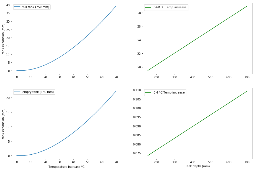
Conclusion¶

It seems that the primary benefit of estimating tank expansion would be to adjust for seasonal increases that occur as the tank gradually changes temperature. However, this is unlikely to have any impact on accumulation data, so it is not worth the expense.

We can see that, at a 5 minute scale, a 6 $^o$C increase would have to exist to create ~0.3 mm (0.01 in) of expansion. A drained tank still holds 62 liters of water, or around 15 gallons. It seems unlikely that the water could be heated or cooled that much over such a short period of time given the high latent heat capacity of water. Since 0.3 mm is the desirable measurement resolution, and around the total instrument error of the LT420, it does not seem that any measurement of accumulated rainfall should be impacted by the expansion of fluid in the tank.

The tank does show 20-30 mm of expansion at max temperature, but that assumes that it is possible to get the entire contents of the tank up to 60 $^o$C. This peak temperature was chosen, because it is the upper peak measured at the stand alone tank orifice. However, it seems unlikely that this temperature is conducted into the water at a substantial enough rate to heat the water to such a high temperature (around the requirements for commercial dishwashers in restaurants). The temperature measurement is taken inbtween 1/2” steel and black fiber-glass, which are both in direct sunlight. While some tank expansion is observed over weeks or months, it does not impact programs that accumulate rainfall.

The addition of a temp sensor is $450 per site, for a project total of $1,350. This expense does not seem justified.